I built a live digit recogniser that runs in your browser. Point a camera at a handwritten number and it tells you which digit it is. The network doing the work is from 1998. It answers in about half a millisecond, and no pixel ever leaves your device.
The model has 61,706 trainable parameters. That is small enough to account for every one of them. A modern image model has hundreds of millions. Nobody checks those by hand, so you end up trusting what you are told. Everything here you can check yourself.
This post builds the whole thing from the bytes up. What MNIST is as a file. What a convolution does to a grid of numbers, and where its weights live. How the 61,706 parameters are split across the layers. What my changes to the 1998 design are worth once you measure them across eleven versions of the model. And why the model gets checked again after it leaves PyTorch.
A mental model you can check against code. The arithmetic itself. Which numbers get multiplied by which. How many of them there are. Why a convolution needs 156 parameters where a dense layer would need 3,692,640 for the same input and output.
An honest answer to a common claim. Modern activations, modern pooling, a modern optimiser, one layer added, one layer taken away. Eleven models, four random seeds each. Nine of the ten changes cannot be told apart from the random seed, and the one that can goes the wrong way. Trained the way the paper describes, with none of the modern pieces, LeNet-5 finishes within one test image of the modern version.
A pipeline you can run. Training takes 91 seconds. The export is checked against all 10,000 test images before it ships. Every number in this post came from that code on my machine.
Sixty Thousand Pictures Behind a Sixteen-Byte Header
MNIST is a set of 70,000 images of handwritten digits, 60,000 for training and 10,000 held back for testing. Everyone uses torchvision.datasets.MNIST and never looks inside. Look inside once, because the format explains the model.
The data ships in a format called IDX, which is about as simple as a binary format gets. Here are the real first sixteen bytes of the training images file, in hexadecimal, where each pair of characters is one byte:
00 00    08     03    00 00 ea 60   00 00 00 1c   00 00 00 1c
└─┬─┘   └┬─┘   └┬─┘   └────┬────┘   └────┬────┘   └────┬────┘
  │      │      │        60000          28            28
  │      │      └──── 3 dimensions
  │      └─────────── 0x08, every value is one unsigned byte
  └────────────────── two zero bytes, always
That is the entire header. Two padding bytes, a type code, a count of dimensions, then one four-byte number per dimension. After byte 16, the pixels start and never stop.
Two things are worth slowing down on.
The numbers are big-endian. A four-byte integer can be written most significant byte first or least significant byte first, and the two conventions disagree completely. Reading 00 00 ea 60 the intended way gives 60,000. Reading the same four bytes backwards gives 1,625,948,160. There is nothing in the file that tells you which convention applies. You have to know, which is why a format always needs a spec alongside it.
If you want to check the arithmetic by hand, each hex digit is a power of 16, counting from the right, and the letters run a=10 through f=15:
$$ \texttt{ea60} = 14 \times 16^3 + 10 \times 16^2 + 6 \times 16^1 + 0 \times 16^0 = 57344 + 2560 + 96 = 60000 $$
Grouping by byte instead of by digit is the same sum rearranged. One byte is two hex digits, so each step left multiplies by $16^2 = 256$: ea is 234, 60 is 96, and $234 \times 256 + 96 = 60000$. Bytes are the natural unit when you are reading a file, so that is usually the easier grouping.
The file size proves the parse. The header is 16 bytes and each image is $28 \times 28 = 784$ bytes, so the file should be exactly $16 + 60000 \times 784 = 47{,}040{,}016$ bytes. It is. Nothing is missing, nothing is left over, and no image is misaligned. That check costs one line and catches an entire family of bugs where an off-by-one in the header offset shifts every image by a few pixels.
The whole reader is seven lines:
import gzip
import struct
import numpy as np

def read_idx(path):
    """IDX: 2 zero bytes, 1 type byte, 1 byte of dimension count,
    then each dimension as a 4-byte big-endian int, then the data."""
    data = gzip.open(path).read()
    ndim = data[3]
    shape = struct.unpack(">" + "I" * ndim, data[4:4 + 4 * ndim])
    return np.frombuffer(data, dtype=np.uint8, offset=4 + 4 * ndim).reshape(shape)
In struct.unpack, the > means big-endian and each I means one four-byte unsigned integer, so ">III" reads three of them. np.frombuffer wraps the existing bytes as an array without copying them, which is why the resulting array is read-only. If you have ever seen PyTorch warn that "the given NumPy array is not writable" while loading MNIST, that warning traces back to exactly this line.
One habit worth keeping: verify the download with a checksum, a short fingerprint computed from the file's contents. A half-finished download still opens without error and still parses, it just quietly contains less data than you think. The four MNIST files have published MD5 checksums, and I confirmed the ones in my copy match the values torchvision ships in its own loader:
train-images-idx3-ubyte.gz       f68b3c2dcbeaaa9fbdd348bbdeb94873
train-labels-idx1-ubyte.gz       d53e105ee54ea40749a09fcbcd1e9432
t10k-images-idx3-ubyte.gz        9fb629c4189551a2d022fa330f9573f3
t10k-labels-idx1-ubyte.gz        ec29112dd5afa0611ce80d1b7f02629c
A checksum you compute from your own download only proves the file will not change later. It becomes meaningful when the expected value comes from somewhere else, so two independent sources have to agree. MD5 is the right tool for catching a truncated download and the wrong tool for catching deliberate tampering, because it is possible to construct two different files with the same MD5. For MNIST that is fine, and it is what the published values use.
The Three Facts That Define the Format
Parse the file and you can measure what an MNIST digit actually looks like. Three statistics matter more than the rest, because the model will come to depend on all three without ever being told about them.
Ink is white, background is black. Pixel values run 0 to 255, and 80.9% of all pixels in the training set are exactly 0. A photograph of a digit on paper is the other way round. Dark ink on a light page. Any real-world image has to be inverted before the model sees it.
The digit always fits a 20 by 20 box. I measured the longest side of the ink's bounding box across all 60,000 training images. It is exactly 20 pixels in 59,987 of them. The remaining 13 come in at 19, and 12 of those are 7s. That is a rounding artefact rather than a coincidence, because MNIST was built this way. The original digit was scaled so its longest side hit 20 pixels, then placed in a 28 by 28 field. The 4-pixel margin is headroom for the next statistic.
The digit is centred by centre of mass at (14, 14). Across those same 60,000 images the mean centre of mass sits at row 14.00, column 14.01, and it moves by only 0.29 either way from image to image. Centre of mass means the average position of the ink weighted by brightness, rather than the centre of the bounding box.
That last distinction is worth doing once with real numbers, because it decides whether your own handwriting will work later.
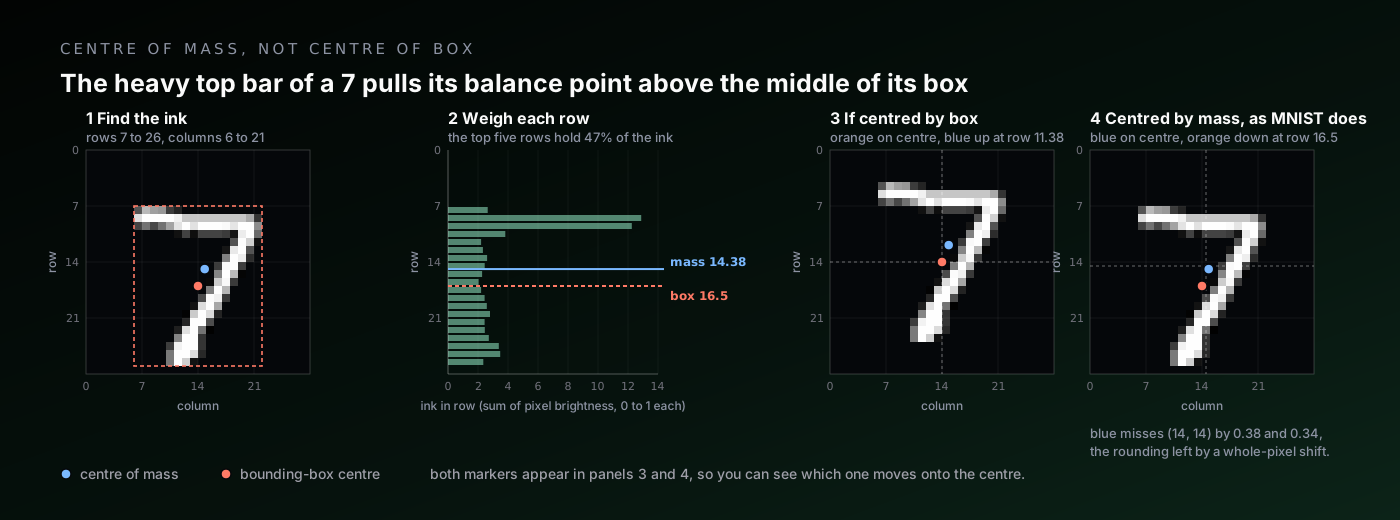
Take the first digit in the test set, a 7. Its ink runs from row 7 to row 26 and column 6 to column 21, so the glyph is 20 tall and 16 wide, and the centre of its box is row 16.5. Now weigh it, treating each pixel's brightness as mass. The top five rows, the bar and its hook, hold 47% of all the ink. The diagonal below is long but thin, about 2.6 units of ink per row. The balance point lands on row 14.38, more than two rows above the centre of the box.
MNIST positions the glyph so that balance point sits at (14, 14). Centring by the box would have put the top edge on row 4. Centring by mass puts it on row 7, three pixels lower, with seven blank rows above and one below.
Two details fall out of that. The target (14, 14) is a pixel index counted from zero, so it sits half a pixel past the true middle of a 28 pixel frame, which is 13.5. And the shift itself is a whole number of pixels, which is why this 7 ends up at 14.38 rather than 14.00. To land it exactly, the crop would have had to start at row 6.62, and there is no such row, so it went to row 7 and the leftover 0.38 stayed. That also explains the spread of 0.29, which is almost exactly $1/\sqrt{12}$, the standard deviation you get from rounding a continuous position to the nearest whole one. Every digit is centred to within half a pixel, and no better.
The classes are also close to balanced, from 5,421 examples of digit 5 to 6,742 of digit 1, so there is no need to reweight anything during training.
Those three facts are the contract. The model will only ever see images that satisfy them, so it will only ever be reliable on images that satisfy them. Most of the work in the browser tool at the end of this post is spent forcing camera frames to comply. A model that scores 99% on MNIST and then fails on real handwriting has usually not been let down by its weights. Nobody enforced the contract at inference time.
Where Are the Weights?
Now the part that actually blocks people, and the reason I wrote this post the way I did.
If you learned neural networks from the standard diagram, you have a specific picture in your head. Circles in columns. Every circle in one column connected to every circle in the next. A weight sitting on each connection, and training nudging those weights. Counting parameters is easy: multiply the two column sizes, add one bias per output.
Then convolution arrives and the explanation changes vocabulary entirely. Filters, kernels, feature maps, sliding windows. The picture of neurons and connections disappears, and nobody says whether it was wrong or just hidden. So the honest question is simple. In that first picture, where are a convolution's weights?
They are exactly where you think. On the connections. A convolution is the same picture with two restrictions added.
Before the wiring, the inputs. An image is a grid of numbers, one per pixel. MNIST gives us 28 by 28 of them, which is 784 inputs and far too many to draw. So take six pixels from a single row and call them x1 to x6. A 0 is background and a 1 is ink. Everything below works the same way at 784 inputs, there is just no way to fit that on a page.
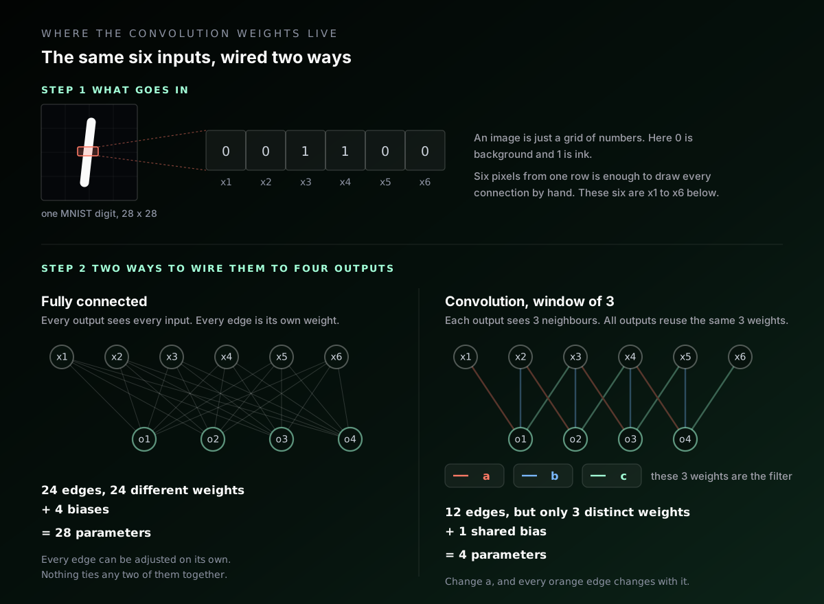
Now wire those six inputs to four outputs. Fully connected, that is $6 \times 4 = 24$ connections, each with its own weight, plus 4 biases. Weights and biases together are the parameters, so 28 of them.
Restriction one: each output only connects to a few neighbouring inputs. Let each output look at a window of three pixels. Output o1 reaches x1, x2, x3, output o2 reaches x2, x3, x4, and so on down the row. The connections that are missing are not weights set to zero and then trained, they simply do not exist. Twelve connections instead of 24.
Restriction two: every output reuses the same weights. Call them $a$, $b$ and $c$. Then:
$$ \begin{aligned} o_1 &= a x_1 + b x_2 + c x_3 + \text{bias} \\ o_2 &= a x_2 + b x_3 + c x_4 + \text{bias} \\ o_3 &= a x_3 + b x_4 + c x_5 + \text{bias} \\ o_4 &= a x_4 + b x_5 + c x_6 + \text{bias} \end{aligned} $$
Same $a$, $b$, $c$ in every row, just applied one position further along. Twelve connections exist, but there are only three distinct weights among them, plus one shared bias. Four parameters, not 28.
That is the rule that makes parameter counting work. A parameter is a distinct value, not a connection. When training adjusts $a$, all four connections carrying $a$ change together, because they are all one number stored in one place.
And "the filter" is nothing more exotic than the list of those shared weights. Saying "a filter of size 3 slides across the input" and saying "every output neuron connects to its own three neighbours using the same three weights" describe the same object. One phrasing emphasises the motion, the other the wiring. The motion is the metaphor. The wiring is what is in memory.
If that still feels like a story rather than a fact, it is checkable. Write the convolution out as a dense weight matrix, one row per output neuron and one column per input, and multiply. For a 4 by 4 input and a 3 by 3 filter producing a 2 by 2 output, that matrix has 64 entries, of which 36 are non-zero and only 9 are distinct:
      x1  x2  x3  x4  x5  x6  x7  x8  x9 x10 x11 x12 x13 x14 x15 x16
o1:    a   b   c   .   d   e   f   .   g   h   i   .   .   .   .   .
o2:    .   a   b   c   .   d   e   f   .   g   h   i   .   .   .   .
o3:    .   .   .   .   a   b   c   .   d   e   f   .   g   h   i   .
o4:    .   .   .   .   .   a   b   c   .   d   e   f   .   g   h   i
I built that matrix explicitly and multiplied it by a random input. It matches F.conv2d on the same input to within floating point error. A convolution is a dense layer whose weight matrix is mostly zeros, with the surviving entries reused across every row. Nothing more mysterious than that.
One Filter, Many Positions
With the wiring settled, the mechanics are arithmetic. At each position the filter covers a patch of the input, multiplies each covered number by its corresponding weight, adds the results, adds the bias, and writes one number to the output.
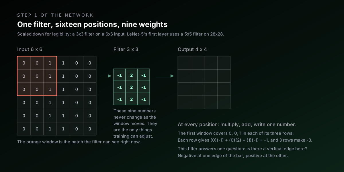
The example in that diagram uses an input with a vertical bar of 1s down the middle of a field of 0s, and a filter whose every row is $[-1, 2, -1]$. Work one position by hand. The leftmost window covers columns 0, 1, 2, which read $0, 0, 1$ in every row. One row contributes $(0)(-1) + (0)(2) + (1)(-1) = -1$, and there are three rows, so the output is $-3$. Slide one step right and the patch becomes $0, 1, 1$, giving $(0)(-1) + (1)(2) + (1)(-1) = +1$ per row, so $+3$.
The full output is $-3, +3, +3, -3$ in every row. The filter is strongly negative at the bar's left edge, strongly positive at its right edge, and would be zero anywhere the input is flat. It answers one narrow question at every location at once: how sharply does brightness change from left to right here?
Two details that trip people up.
The output is smaller than the input, unless you pad. A 3 by 3 filter on a 6 by 6 input only has 4 valid positions per axis, because the filter has to fit entirely inside. In general a $k \times k$ filter turns an $n \times n$ input into $(n - k + 1)^2$ outputs. LeNet-5's first layer uses a 5 by 5 filter on a 28 by 28 image, which would give 24 by 24. I pad the input with 2 pixels of zeros on every side so the output stays 28 by 28, which is the modern convention and keeps the arithmetic tidy.
Frameworks do not flip the filter. Textbook convolution reverses the filter before multiplying. PyTorch's conv2d, like almost every deep learning framework, skips the flip and computes what mathematicians call cross-correlation. Since the weights are learned anyway, the network simply learns the flipped version if that is what it needs, and nobody notices. It matters only if you are hand-building a filter and expecting a specific sign.
Stacking Filters, and What a Channel Is
One filter produces one output grid. That grid is called a feature map, and it records how strongly that one filter responded at every location.
Detecting only vertical edges is not much of a vision system, so a layer uses several filters. Six filters produce six feature maps, each from its own independent set of weights. Nothing is shared between filters.
Now the input to the next layer is six grids rather than one. This is where the counting gets its one genuinely new rule: a filter must have one slice for every input grid. If a layer receives 6 feature maps and uses 5 by 5 filters, then each of its filters is a stack of 6 separate 5 by 5 grids of weights, a total of 150 numbers. Each slice is applied to its matching input grid, and the results are added together into a single output grid.
So the general formula is:
$$ \text{params} = \underbrace{F}_{\text{filters}} \times \Big( \underbrace{C}_{\text{input maps}} \times k \times k + \underbrace{1}_{\text{bias}} \Big) $$
More filters means more output maps. More input maps means thicker filters and more numbers added into each output. That single formula accounts for every convolutional parameter in the network.
Pooling, or Discarding Three Quarters on Purpose
Between convolutions sits a pooling layer, which shrinks each feature map by summarising small neighbourhoods. With 2 by 2 max pooling, every non-overlapping 2 by 2 block is replaced by its largest value, so a 28 by 28 map becomes 14 by 14 and three quarters of the numbers are gone.
Pooling has no parameters at all, neither weights nor a bias. It is a fixed rule, so there is nothing for training to adjust.
It buys two things. The obvious one is cost: everything downstream operates on a quarter as many numbers. The subtler one is that it makes the network slightly indifferent to exact position. If a stroke shifts by one pixel, the maximum within its block is often unchanged, so the summary is unchanged. For reading handwriting, where nobody writes the same 4 twice, a little positional indifference is exactly what you want.
Shrinking the grid also widens what each later unit can see. The receptive field of a unit is the region of the original image that can influence it. I measured it by backpropagating a one into a single unit and checking which input pixels received gradient:
| After | Output shape | Receptive field |
|---|---|---|
| C1 conv | 6 x 28 x 28 | 5 x 5 |
| S2 pool | 6 x 14 x 14 | 6 x 6 |
| C3 conv | 16 x 10 x 10 | 14 x 14 |
| S4 pool | 16 x 5 x 5 | 16 x 16 |
A unit in the first layer sees a 5 by 5 patch, about the size of a stroke fragment. By the second convolution a unit sees 14 by 14, half the image, enough for a loop or the junction of a 4. The network builds from strokes to parts without anyone specifying what a stroke or a part is.
The Full Architecture, Layer by Layer
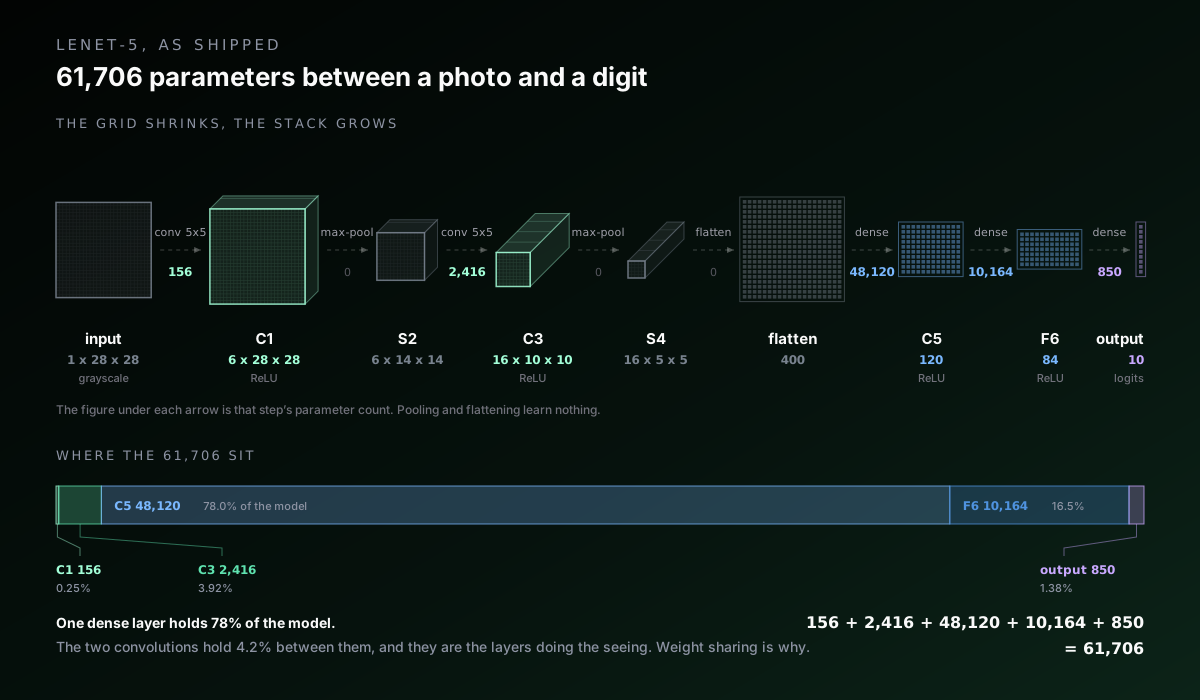
Here is the whole network. Each tensor is drawn to scale, so you can watch the square shrink while the stack behind it deepens. The parameter counts sit on the arrows rather than on the boxes, because that is where they live: a weight belongs to the step from one tensor to the next, not to either tensor. Pooling and flattening therefore read zero.
In PyTorch the definition is short enough to read in one pass:
import torch.nn as nn

class LeNet5(nn.Module):
    def __init__(self, num_classes: int = 10):
        super().__init__()
        self.features = nn.Sequential(
            nn.Conv2d(1, 6, kernel_size=5, padding=2),   # 1 x 28 x 28 -> 6 x 28 x 28
            nn.ReLU(inplace=True),
            nn.MaxPool2d(2),                             #            -> 6 x 14 x 14
            nn.Conv2d(6, 16, kernel_size=5),             #            -> 16 x 10 x 10
            nn.ReLU(inplace=True),
            nn.MaxPool2d(2),                             #            -> 16 x 5 x 5
        )
        self.classifier = nn.Sequential(
            nn.Flatten(),                                #            -> 400
            nn.Linear(16 * 5 * 5, 120),
            nn.ReLU(inplace=True),
            nn.Linear(120, 84),
            nn.ReLU(inplace=True),
            nn.Linear(84, num_classes),                  #            -> 10
        )

    def forward(self, x):
        return self.classifier(self.features(x))
The last layer returns ten raw scores called logits, one per digit. They are not probabilities and can be negative. Turning them into probabilities means exponentiating each and dividing by the total, which is the softmax function. I deliberately leave softmax out of the model, for a reason that matters at export time and that I will come back to.
Counting the 61,706
Apply the formula layer by layer.
| Layer | Shape in | Shape out | Calculation | Parameters |
|---|---|---|---|---|
| C1 conv | 1 x 28 x 28 | 6 x 28 x 28 | 6 x (1 x 5 x 5 + 1) | 156 |
| S2 pool | 6 x 28 x 28 | 6 x 14 x 14 | fixed rule | 0 |
| C3 conv | 6 x 14 x 14 | 16 x 10 x 10 | 16 x (6 x 5 x 5 + 1) | 2,416 |
| S4 pool | 16 x 10 x 10 | 16 x 5 x 5 | fixed rule | 0 |
| C5 dense | 400 | 120 | 120 x (400 + 1) | 48,120 |
| F6 dense | 120 | 84 | 84 x (120 + 1) | 10,164 |
| Output | 84 | 10 | 10 x (84 + 1) | 850 |
| Total | 61,706 |
Two things in that table are worth sitting with.
The convolutions are almost free, and do almost all the work. C1 and C3 together hold 2,572 parameters, 4.2% of the model. C5 alone holds 78%. But counting multiply-accumulate operations for a single image instead of parameters reverses the picture completely:
| Layer | Multiply-accumulates | Share of compute | Share of parameters |
|---|---|---|---|
| C1 conv | 117,600 | 28.2% | 0.3% |
| C3 conv | 240,000 | 57.6% | 3.9% |
| C5 dense | 48,000 | 11.5% | 78.0% |
| F6 dense | 10,080 | 2.4% | 16.5% |
| Output | 840 | 0.2% | 1.4% |
The two convolutions are 4.2% of the parameters and 85.9% of the arithmetic. That is weight sharing stated as a ratio. The same 156 parameters get reused across 784 positions, so a tiny amount of memory drives a large amount of computation. The dense layers are the opposite, a large amount of memory used exactly once each.
Weight sharing is doing enormous work in C1. That layer maps 784 input values to $6 \times 28 \times 28 = 4{,}704$ output values. Count it three ways:
| How you count C1 | Number |
|---|---|
| A fully connected layer between the same two sets of neurons | 3,692,640 |
| Connections that actually exist in the convolution | 117,600 |
| Distinct parameters in the convolution | 156 |
Same inputs, same outputs, 23,671 times fewer parameters. That ratio is the entire reason convolutional networks work on images with modest data and modest hardware. A fully connected first layer would have to learn what a stroke looks like separately at every one of 784 positions. Nothing it learned in the top left corner would transfer to the bottom right. The convolution learns it once and applies it everywhere.
What I Changed From 1998
The architecture above is LeNet-5 as published, with the original layer shapes and therefore the original parameter count, but three substitutions that are now standard. Two of them are in the network. The third is how the network was trained.
Activations: tanh became ReLU. An activation function is the nonlinearity applied after each layer, and without one a stack of layers collapses into a single linear layer no matter how deep it is. The 1998 network used $\tanh$, which squashes any input into the range $[-1, 1]$. The modern default is ReLU, the rectified linear unit, which is just $\max(0, x)$: negatives become zero and positives pass through unchanged.
The textbook argument for ReLU is gradient flow. $\tanh$ flattens out at both ends, so a unit with a large input has a derivative near zero and receives almost no gradient. Stack enough of those and the signal reaching the early layers vanishes. ReLU's derivative is exactly 1 for every positive input, so gradient passes through undiminished however deep the stack gets.
Pooling: average became max. The original paper used average pooling with a trainable coefficient per map. I use plain max pooling, which keeps the strongest response in each block rather than blending the block together. The intuition is that for detecting whether a feature is present, the peak response carries the signal and averaging it with three neighbours dilutes it.
The optimiser: hand-tuned SGD became Adam. The optimiser is the rule that turns a gradient into an actual change in the parameters. LeCun trained LeNet-5 with plain stochastic gradient descent and backpropagation, with per parameter step sizes estimated by a stochastic diagonal Levenberg-Marquardt method, and a global learning rate lowered by hand as the run progressed. I use Adam, which keeps a running average of each parameter's recent gradients and of their recent sizes, then sets that parameter's step from the two. It needs no schedule written by hand, which is most of why it became the default.
None of the three changes the parameter count, since activations, pooling rules and optimisers hold no weights of their own. All three get repeated constantly as obvious improvements. So I measured them.
What the Change Was Actually Worth
I trained all four combinations under identical conditions: same initialisation seed, same data order, same optimiser, same eight epochs. Then I repeated the whole thing across four different seeds, because a single run cannot tell you whether a gap is real or just where the random number generator happened to land. Every figure below is test accuracy after the eighth epoch, and bold marks the best run in each seed column.
| Variant | seed 1998 | seed 7 | seed 42 | seed 2024 | Mean |
|---|---|---|---|---|---|
| 1998 activations: tanh + average pool | 98.92% | 98.80% | 99.08% | 98.93% | 98.93% |
| tanh + max pool | 98.85% | 98.99% | 98.93% | 98.81% | 98.89% |
| ReLU + average pool | 98.96% | 98.96% | 99.00% | 98.89% | 98.95% |
| shipped: ReLU + max pool | 99.05% | 98.89% | 98.99% | 98.95% | 98.97% |
The modern pair averages 98.97% and the 1998 pair averages 98.93%. That is a gap of 0.037 percentage points, which on 10,000 test images is about four images.
Now compare that to how much a single variant moves when you change nothing but the seed. The 1998 configuration ranges from 98.80% to 99.08% across its four runs, a spread of 0.28 points. The gap between the shipped configuration and the 1998 activations is roughly seven times smaller than the variation within one variant.
Every one of the sixteen runs lands between 98.80% and 99.08%. The highest single score among them, 99.08%, belongs to the 1998 activations. The shipped configuration beats the original on three seeds out of four and loses on the fourth. There is no effect here to report.
The theoretical argument for ReLU is about deep networks. LeNet-5 is five layers deep. Vanishing gradients through $\tanh$ are a real problem at twenty layers and a mild one at five, so the thing ReLU is best at barely gets to matter here. Adam, the optimiser, adapts its step size per parameter, and I assumed it was papering over a good deal of what the activation choice would otherwise cost. It is not, and there is a later section that takes Adam away to check. The 1998 design was not holding anything back on this problem.
I kept ReLU and max pooling anyway, for reasons that are honest but have nothing to do with accuracy. They are the modern default, so the code reads as familiar. ReLU also exports to a cheaper operation for browser inference. What I will not claim is that they bought accuracy, because measured properly, on this problem, they did not.
One Layer More, One Layer Less
Swapping the activation changes the rule each layer computes by. The other knob people reach for first is how many layers there are at all. So I ran the same experiment on depth: take the shipped model, remove exactly one layer or add exactly one, leave everything else alone, and train it across the same four seeds.
The baseline here is the shipped model itself, with nothing altered. Both scripts build it from the same layer list and reseed before constructing it, so it starts from the same weights and returns the same logits as the model the tool runs. I checked that rather than assuming it, and it is why the baseline row reproduces the earlier table exactly.
Using the layer names from the counting table above, here is what each variant does.
C3 removed takes S4 with it. Pooling has no parameters. A pooling step with no convolution feeding it is also not something anyone writes on purpose, so the second convolutional stage comes out whole and C5 ends up reading the output of S2.
F6 removed leaves C5 feeding Output. The 84 unit layer comes out and the 120 unit layer connects straight to the ten logits.
The added convolution sits after S4. It is a 3 by 3 filter, 16 channels in and 16 out, with one pixel of padding so the feature maps stay 5 by 5. The flatten still arrives at 400, every layer after it is untouched, and the only parameters the model gains are the new layer's own.
The added dense layer sits after F6. A second 84 unit layer goes between F6 and Output, which keeps the output head itself unchanged.
Here is what each variant costs before a single image goes through it.
| Variant | Exactly what changed | Parameters | vs shipped |
|---|---|---|---|
| shipped, unchanged | C1, S2, C3, S4, C5, F6, Output | 61,706 | reference |
| C3 removed, with S4 | the second convolution and its pooling come out, so C5 receives 6 x 14 x 14 | 152,410 | 90,704 more |
| F6 removed | the 84 unit layer comes out, C5 feeds Output directly | 51,902 | 9,804 fewer |
| convolution added after S4 | a third convolution sits between S4 and the flatten, 16 channels to 16, 3 by 3, padded | 64,026 | 2,320 more |
| dense layer added after F6 | a second 84 unit layer sits between F6 and Output | 68,846 | 7,140 more |
The first row is the surprise, and it needs no training run to see. Taking a layer out makes this model nearly two and a half times larger.
The second convolution is what shrinks the picture from 14 by 14 down to 5 by 5 before the flatten. Remove it and the flatten arrives at 6 channels of 14 by 14, which is 1,176 numbers rather than 400. The first fully connected layer grows from 48,120 parameters to 141,240 to meet it. In a network that ends in fully connected layers, depth and size can move in opposite directions.
Then the accuracy, same protocol as before. Four seeds, eight epochs, test accuracy after the eighth, bold marks the best run in each seed column.
| Variant | seed 1998 | seed 7 | seed 42 | seed 2024 | Mean |
|---|---|---|---|---|---|
| shipped, unchanged | 99.05% | 98.89% | 98.99% | 98.95% | 98.97% |
| C3 removed, with S4 | 98.72% | 98.65% | 98.76% | 98.75% | 98.72% |
| F6 removed | 98.90% | 99.00% | 98.97% | 99.18% | 99.01% |
| convolution added after S4 | 98.96% | 98.95% | 98.75% | 98.83% | 98.87% |
| dense layer added after F6 | 98.88% | 99.00% | 98.79% | 99.03% | 98.92% |
One row moves, and it moves for real. Removing C3 costs 0.25 points, and it is the only result anywhere in this post where a variant's four runs sit entirely outside the baseline's four runs. The worst shipped seed is 98.89% and the best C3-removed seed is 98.76%, so the two sets do not overlap at any point. Shuffle those eight runs into two groups of four every way possible, all seventy of them, and a split this clean comes up 2 times, which puts it at p = 0.029. That is the smallest value four against four can produce.
The other three changes are smaller than the wobble between seeds. Removing F6 finishes 0.043 points ahead while its own four runs span 0.28 points, the extra convolution after S4 lands 0.097 behind, the extra dense layer after F6 lands 0.045 behind, and all three overlap the baseline's range. The same permutation test returns 0.60, 0.20 and 0.51 for them.
Put the two columns together and the shape of the result is uncomfortable for the usual intuitions. The change that hurt is the change that added 90,704 parameters. The change that removed 9,804 parameters cost nothing anyone could measure.
The Optimiser Nobody Was Varying
Both experiments above hold the optimiser fixed, and that optimiser is Adam, published in 2014. So the row labelled 1998 in those tables is the 1998 layer choices trained the modern way. The comparison was never tanh against ReLU on equal terms. It was tanh plus Adam against ReLU plus Adam, which leaves the recipe LeCun actually used untested.
What he used was plain stochastic gradient descent: compute the gradient on a batch, step every parameter a little way against it, repeat. The paper adds a per parameter step size estimated by a method called stochastic diagonal Levenberg-Marquardt, and a global rate the authors lowered by hand as training progressed. Adam does that scheduling for you, which is most of why it won.
A learning rate that suits Adam does not suit SGD. Adam's 0.001 would barely move plain SGD in eight epochs, and beating a method because its step size was wrong proves nothing about the method. So I swept the rate on one seed first, then carried the winner into the real runs.
| Optimiser | Learning rate | Test accuracy after 8 epochs |
|---|---|---|
| plain SGD | 0.01 | 97.73% |
| plain SGD | 0.03 | 98.45% |
| plain SGD | 0.1 | 99.01% |
| plain SGD | 0.3 | 99.14% |
| plain SGD | 0.5 | 9.80% |
| plain SGD | 1.0 | 9.80% |
| SGD, momentum 0.9 | 0.003 | 98.75% |
| SGD, momentum 0.9 | 0.01 | 98.78% |
| SGD, momentum 0.9 | 0.03 | 99.06% |
| SGD, momentum 0.9 | 0.1 | 98.15% |
Plain SGD improves up to 0.3 and then falls off a cliff. At 0.5 and above the run diverges and finishes at 9.80%, which is roughly what you score by guessing. So 0.3 is a real peak rather than the edge of whatever grid I happened to try. Momentum peaked at 0.03. Both rates were chosen on seed 1998 alone and Adam was left at the repo's default of 0.001, so if this test is tilted, it is tilted towards SGD.
Then the same protocol as the other two experiments: four seeds, eight epochs, same data order within a seed.
| Variant | seed 1998 | seed 7 | seed 42 | seed 2024 | Mean | Spread |
|---|---|---|---|---|---|---|
| shipped: ReLU, max pool, Adam | 99.05% | 98.89% | 98.99% | 98.95% | 98.97% | 0.16 |
| SGD with momentum 0.9, lr 0.03 | 99.06% | 98.76% | 98.17% | 99.15% | 98.78% | 0.98 |
| plain SGD, lr 0.3 | 99.14% | 98.95% | 98.52% | 99.08% | 98.92% | 0.62 |
| the whole 1998 recipe: tanh, average pool, plain SGD | 99.06% | 98.92% | 99.06% | 98.88% | 98.98% | 0.18 |
The last row is the one I was after. Take the published activations, the published pooling rule and gradient descent with none of Adam's machinery, and the result averages 98.98% against the fully modern 98.97%. On 10,000 test images that difference is one image, and it favours 1998.
That also closes a loose end from earlier. I had said Adam adapts its step size per parameter and papers over much of what the activation choice would otherwise cost. If that were true, taking Adam away should have exposed tanh. It does not. Under plain SGD, tanh with average pooling scores 98.98% and ReLU with max pooling scores 98.92%. The activation result replicates under a different optimiser, which is more than I expected to be able to say about it.
One thing here does separate, and it is not the mean. It is the spread. Adam's four runs sit inside 0.16 points. Plain SGD spans 0.62 points and SGD with momentum spans 0.98, which is six times Adam's range. Seed 42 is where both SGD variants fall over, at 98.52% and 98.17%. Some of that is likely the rate itself, since it was tuned on seed 1998 and a rate that suits one seed need not suit another. That is the finding rather than an excuse for it. Adam at an untouched default was the most predictable of the four, and predictability does not show up in a mean.
By the permutation test used earlier, none of the three optimiser changes separates from the shipped model: p = 0.57 for momentum, and 0.91 for both plain SGD and the full 1998 recipe.
All Eleven Models, Side by Side
All three experiments include the shipped configuration, and all three reseed before building each model, so the shipped rows are not merely close across the three scripts. Seed by seed and epoch by epoch, they are the same numbers. That is worth stating because it is what makes the three tables comparable rather than merely adjacent.
So here is every model this post trained, with the reason I tried it, what it cost, and what it did.
The last two columns are the ones that decide anything, so they are worth a sentence each.
Spread over its own four runs is the model arguing with itself. Train one architecture four times with four different random seeds and you get four different scores, because the starting weights and the order the images arrive in are both drawn at random. This column is the best of those four minus the worst, in percentage points.
Clear of that spread asks whether the gap to the shipped model is bigger than the model's own disagreement with itself.
Take the F6 row as the worked example. Its four seeds scored 98.90%, 99.00%, 98.97% and 99.18%. Nothing separates those runs except the random number generator, and they already span 0.28 points. Its average lands 0.043 points above the shipped model. The effect being claimed is about six times smaller than the measurement's own wobble, so the honest answer is that the change has not been shown to do anything.
| Change | Why I tried it | Parameters | Mean | Gap to shipped | Spread over its own four runs | Clear of that spread? |
|---|---|---|---|---|---|---|
| shipped, unchanged: ReLU, max pool, C1 to Output | the configuration the tool runs | 61,706 | 98.97% | reference | 0.16 points | reference |
| tanh and average pool (1998 activations) | the published activation and pooling | 61,706 | 98.93% | 0.037 behind | 0.28 points | no |
| tanh, max pool | isolates the activation | 61,706 | 98.89% | 0.075 behind | 0.18 points | no |
| ReLU, average pool | isolates the pooling rule | 61,706 | 98.95% | 0.017 behind | 0.11 points | no |
| C3 removed, with its S4 pooling | fewer stages should be cheaper | 152,410 | 98.72% | 0.250 behind | 0.11 points | yes, worse on all four seeds |
| F6 removed, C5 feeds Output | the head looked redundant | 51,902 | 99.01% | 0.043 ahead | 0.28 points | no |
| convolution added after S4 | more stages should extract more | 64,026 | 98.87% | 0.097 behind | 0.21 points | no |
| second 84 unit layer after F6 | more mixing capacity | 68,846 | 98.92% | 0.045 behind | 0.24 points | no |
| SGD with momentum 0.9, lr 0.03 | the optimiser was never varied | 61,706 | 98.78% | 0.185 behind | 0.98 points | no |
| plain SGD, lr 0.3 | the method the paper used | 61,706 | 98.92% | 0.047 behind | 0.62 points | no |
| the whole 1998 recipe at once | tanh, average pool and plain SGD together | 61,706 | 98.98% | 0.010 ahead | 0.18 points | no |
Read the gap column against the spread column and the table answers itself. Only one row has a gap bigger than its own wobble, and the gap goes the wrong way.
Five things fall out of reading that table across rather than down.
Accuracy. Ten changes were tested and one of them registered. Everything else sits inside a band roughly 0.2 points wide, and 0.2 points is also how far a single unchanged configuration wanders when you rerun it on a different seed. The honest summary of six of these seven experiments is that they found nothing, and that is a result rather than a failure to get one.
Parameters. The parameter column and the accuracy column barely speak to each other. The largest model by a wide margin, at 152,410 parameters, is the worst one. The smallest, at 51,902, is nominally the best, though not by enough to claim. Across the range from 51,902 to 68,846 the accuracy moves less than a tenth of a point. MNIST at this scale is saturated, and extra capacity has nothing left to buy.
Rationale against outcome. Every change in that table has a textbook argument behind it. ReLU for gradient flow, max pooling for peak response, more layers for more abstraction, fewer layers for less cost. Nine of the ten arguments produced no measurable effect on this problem. The seventh produced one, and it ran against the intuition that removing a layer gives you a smaller, cheaper model.
Consistency, which the mean hides. The three optimiser rows all land within a fifth of a point of the shipped mean, but they do not get there as reliably. Adam's runs span 0.16 points, plain SGD's span 0.62 and momentum's span 0.98. Two models can be equally accurate on average and still differ in how much the seed is allowed to decide, and only the spread column shows it.
What the one real result is actually saying. The convolution layers are the ones that matter. Remove C3 and accuracy drops even though the parameter count nearly triples, because the replacement capacity arrives as a fully connected layer that has to learn each position separately. That is the 23,671 to 1 comparison from earlier in this post showing up as an accuracy number instead of an arithmetic one. The dense head, meanwhile, can lose a whole layer without anyone noticing.
Training It
The training script is ordinary, which is the point. The interesting decisions are in the data and the architecture, not the loop.
train_tf = transforms.Compose([
    transforms.RandomAffine(degrees=10, translate=(0.1, 0.1), scale=(0.9, 1.1)),
    transforms.ToTensor(),
    transforms.Normalize((0.1307,), (0.3081,)),
])
Three things happen to every training image.
Mild affine jitter. Each image is randomly rotated up to 10 degrees, shifted up to 10%, and scaled between 0.9 and 1.1. This is data augmentation: making slightly altered copies so the model sees more variety than the dataset literally contains. The amounts are deliberately small, because the preprocessing in the browser already centres and scales the digit the way MNIST does. The variation left to cover is the wobble in how somebody writes, not large transformations that preprocessing will remove anyway.
Conversion to floats in $[0, 1]$. Pixels are stored as bytes to keep the training images at 47 MB, and converted only at training time.
Normalisation. Subtract 0.1307 and divide by 0.3081, the mean and standard deviation of MNIST pixel values. This centres the inputs near zero with a spread near one, which is the range optimisers are tuned for. Those two constants have to be applied identically at inference, and getting them wrong there is a classic silent failure: the model still runs, still outputs confident answers, and is quietly worse.
The loop itself is Adam at a learning rate of 0.001, a batch size of 128, cross-entropy loss, and a cosine schedule that anneals the learning rate towards zero across the run. After each epoch the model is evaluated on the 10,000 test images and the best one is saved.
device: mps
parameters: 61,706
epoch  1/15  train_loss 0.5458  test_loss 0.0953  test_acc 96.91%  11.0s
epoch  5/15  train_loss 0.0866  test_loss 0.0402  test_acc 98.58%   5.7s
epoch 10/15  train_loss 0.0546  test_loss 0.0299  test_acc 99.03%   5.7s
epoch 14/15  train_loss 0.0436  test_loss 0.0205  test_acc 99.30%   5.8s
epoch 15/15  train_loss 0.0419  test_loss 0.0205  test_acc 99.27%   5.8s

best test accuracy: 99.30%  (90.9s total)
Ninety one seconds on an M4's GPU through PyTorch's mps backend, for 99.30% on data the model never trained on. It is worth pausing on how little that costs now. Hardware has moved much further since then than this architecture has.
One caveat about that number, since this post is partly about not overclaiming. The 10,000 test images were used to pick which epoch to keep. That makes 99.30% very slightly optimistic as an estimate of performance on genuinely unseen data, because the test set influenced one decision. The clean version uses a third split for model selection. At this scale the effect is small, but it is the kind of thing worth saying out loud rather than discovering in the comments.
Exporting to ONNX, and Why I Check It Afterwards
The browser cannot run PyTorch, so the trained model is converted to ONNX, a portable format that describes a network as a graph of standard operations. Lots of runtimes can read it, including one that runs in a browser tab.
torch.onnx.export(
    model,
    (torch.zeros(1, 1, 28, 28),),
    "lenet5.onnx",
    input_names=["input"],
    output_names=["logits"],
    dynamic_axes={"input": {0: "batch"}, "logits": {0: "batch"}},
    opset_version=13,
)
The result is a 243 KB file, and almost all of it is the parameters themselves. 61,706 of them at 4 bytes each is 241 KB, which leaves 2,485 bytes for the graph: the list of operations, their order, and the shapes flowing between them.
Now the part most tutorials skip. Export is a translation between two systems with different internal conventions, and translations can change behaviour: operations get fused, a padding convention is interpreted differently, a dtype is silently narrowed. The failure mode is nasty precisely because it is quiet. The model looks fine in Python, and misclassifies in the browser, and nothing anywhere reports an error.
So the export script runs both models over all 10,000 test images and compares their raw outputs:
torch_logits = model(images).numpy()
onnx_logits = session.run(["logits"], {"input": images.numpy()})[0]

max_abs_diff = max(max_abs_diff, float(np.abs(torch_logits - onnx_logits).max()))
label_mismatches += int((torch_logits.argmax(1) != onnx_logits.argmax(1)).sum())
parity check
samples 10000
max abs logit diff 1.335e-05 (tolerance 1e-04)
prediction mismatches 0
pytorch accuracy 99.30%
onnx accuracy 99.30%
result PASSZero disagreements out of ten thousand, and the largest difference between any two corresponding logits is 1.3 in the fifth decimal place, which is ordinary floating point drift from operations being reordered. If either check failed the script exits non-zero and the file does not ship.
This is also where leaving softmax out of the model pays off. Comparing logits compares the model's actual output. Softmax squashes everything into $[0, 1]$ and compresses differences, so two models that genuinely disagree can look similar after it. Comparing before the squashing makes the check strictly more sensitive. The browser applies softmax afterwards, where a discrepancy cannot hide.
Writing the accuracy into a small JSON file next to the model is a related habit. The page reads its "99.30%" from that file rather than from hardcoded text, so the number on screen always belongs to the model actually being served. Retrain, and the page updates itself or it does not change at all. It cannot drift into being confidently wrong.
What the Browser Tool Actually Does
The tool is the same 61,706 parameters, running in a worker thread through ONNX Runtime Web. Two parts are worth describing, because between them they are most of the difficulty.
Preprocessing is where accuracy is won or lost. The model only ever saw images obeying the three statistics from earlier. A camera frame obeys none of them. So every frame goes through six steps before a single weight is touched.
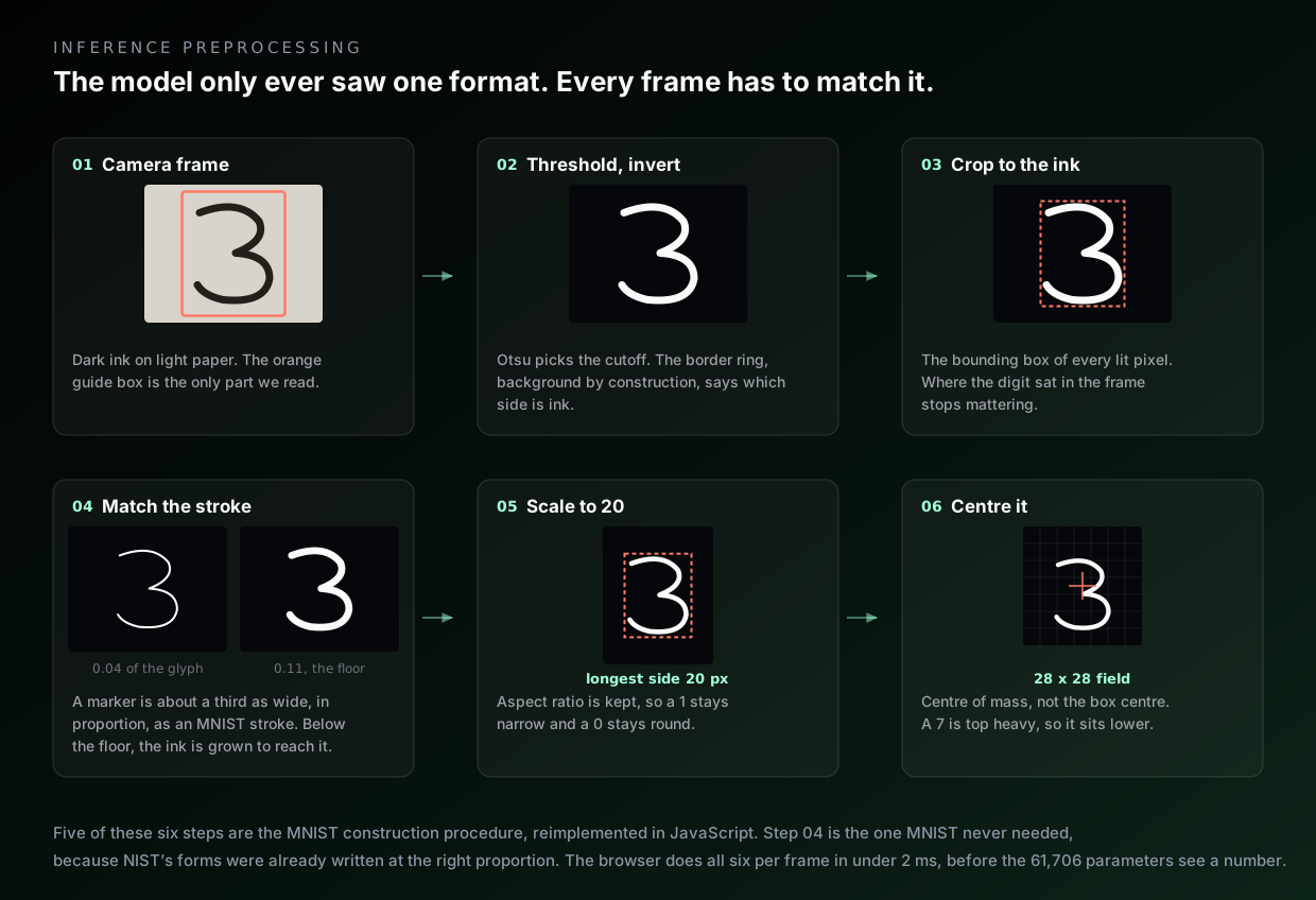
The frame is cropped to the guide box. A threshold separates ink from paper, chosen automatically by Otsu's method, which picks the cutoff that best splits the pixel histogram into two groups. Polarity is decided by looking at the border ring of the crop, which is background by construction, so if the border is the bright side then the ink is dark and the image gets inverted. The image is cropped tight to the ink's bounding box, which removes any dependence on where the digit sat in frame. The stroke is measured and, if it is thinner than MNIST's, thickened to match. It is then scaled so its longest side is 20 pixels, preserving aspect ratio so a 1 stays narrow and a 0 stays round. Finally it is placed into a 28 by 28 field positioned so its centre of mass lands at the centre.
Three details in that list are worth more than they look, because all three were bugs before they were features.
The first is that the ink has to be rescaled by its own peak, not by the full 0 to 255 range. A camera never sees pure black ink on a pure white page: marker reads around 40 to 70, and cream paper closer to 200 than 255. Scale against the theoretical range and the stroke arrives at roughly half brightness, while every MNIST digit has a fully saturated core. The network is then being asked about something it has never seen. Measured on a synthetic page, the stroke reached the model at a peak of 142 out of 255 instead of 255, and confidence fell with the light. Rescaling by the ink's own 99th percentile, rather than its maximum so one specular highlight cannot set the range, puts it back at 255.
The second is that Otsu finds the strongest boundary in the frame, which is not always the one you want. Hold a sheet of paper that does not fill the guide box and the strongest boundary is desk against page, not ink against page. What comes back is the sheet itself, a solid block the network reads as some bold, blobby digit, which is the failure you see as a confident wrong answer that ignores your writing. The tell is geometric: a stroke never fills its own bounding box, and a surface nearly does. Measuring all ten digits at three stroke widths, the worst genuine case was a thick 1, whose box is a narrow slab filled to 0.74, over an area of 0.11 of the frame. A page sits near 0.89 over 0.21 or more. When both numbers say surface, the preprocessor looks again inside that region, where the only two levels left are paper and ink.
The third is that a stroke can be the right shape and still the wrong width. An MNIST stroke is about 3 pixels across in a 20 pixel glyph, a ratio of 0.15. Measured on a photo of a 4 drawn in marker, the stroke was 29 pixels across a 667 pixel glyph, which is 0.044. Scale the longest side down to 20 and a stroke that thin arrives under a pixel wide, so the averaging in the rescale smears it to grey. Of the lit pixels that reached the model, 0 to 2% were above 0.9 brightness. In MNIST the figure is 50%. Every MNIST digit has a saturated core and this one had none. The drawing canvas never hit this, because 26 pixels of line on a 250 pixel digit is already 0.10, which is close enough. The fix is to measure the median stroke run and grow the ink when it falls below 0.11 of the glyph's longest side. That took the photo from 77 to 83% confidence up to 92 to 96%, held the drawing canvas at 100%, and left accuracy on 1,000 real MNIST digits pushed through the same pipeline unchanged at 98.4%. The floor is 0.11 rather than MNIST's own 0.15 because at 0.13 the filter starts firing on a quarter of real MNIST digits and costs accuracy.
That ratio depends on your pen, your paper and your light, so 0.11 is a sensible default and a poor fixed rule. The camera panel carries a slider for it, and reports what the current frame measured. Drag the floor down to zero while holding a thin digit and you can watch the confidence fall, then drag it back and watch the stroke thicken and the answer firm up.
None of these are arbitrary. The six steps are the MNIST construction procedure reimplemented in JavaScript, with one addition, because a camera does not hand you what a 1990s scanner handed NIST. The only way to make a model work on new data is to give it something shaped like what it trained on.
The runtime sits in a worker. A worker is a separate thread, so inference never blocks the camera loop or the interface. Each frame posts a 784-number array across, gets back ten probabilities, and the main thread stays free to draw. Inference takes 0.5 to 1.0 ms and preprocessing 1.6 to 1.9 ms, so the budget is dominated by getting the image into shape rather than by the network.
Two small behaviours came out of testing rather than design. The first is that drawing updates arriving while an inference is in flight were being dropped, so the readout could describe a stroke you had already finished changing. The fix is to remember that a newer version exists and re-run as soon as the worker frees up. The second involves the smoothing that steadies the live camera reading, an exponential average over recent frames. That averaging is actively wrong for the drawing canvas, where each update is a genuinely different shape rather than a noisy repeat of the same one. It now smooths the camera only. Both bugs looked like model problems and were not.
Where This Leaves the Model
LeNet-5 at 99.30% on MNIST is a solved problem and has been for a long time. The reason to build it is legibility. At 61,706 parameters every design decision can still be checked. You can count the parameters, measure the receptive field, verify by direct computation that a convolution is a weight-shared dense layer, and test whether a change you made was worth anything. None of those are available to you on a model with 400 million parameters, and the intuitions you build here are the ones you carry there.
The honest summary of what the investigation turned up is this. The architecture does the heavy lifting, and weight sharing is what makes that possible: 156 parameters doing a job that would otherwise take 3.7 million. The modernisations I made on top of the 1998 design are defensible on other grounds but did not buy accuracy, and neither did a deeper head nor a thinner one. Nor did Adam: assemble the whole published recipe, tanh and average pooling and plain gradient descent, and it finishes level with the modern build. One change out of ten registered at all, and it was removing a convolution, which cost a quarter of a point while nearly tripling the parameter count. I only know any of that because I measured across seeds instead of running once. The preprocessing is half the system, and it is the half that decides whether the thing works on real handwriting. And the export needs checking, because the one failure mode that will genuinely cost you a weekend is the one that reports success at every step.
The tool is here, and the training, export and ablation scripts are in the same folder as the page itself. Point a camera at something you wrote and watch a network from 1998 read it.